Universal Correlation Coefficient

(Available in R or Python.)

At the 2011 Joint Statistical Meetings, Nuo Xu of the University of Alabama at Birmingham presented a paper--coauthored with Xuan Huang also of UAB and Samuel Huang at the University of Cincinatti--in which a Universal Correlation Coefficient is defined and developed. For two discrete random variables `x` and `y`, this coefficient gives the degree of dependency, but not the form of dependency.

I've created an R library for calculating this coefficient. This coefficient is useful for programmatically determining, amongst several discrete random variables, which pairs have (potentially non-linear) relationships.

Huh? Coefficient of what?

Recall that the Pearson Correlation Coefficient `r` is a number between -1 and 1 that represents how close your data is to fitting on a line:

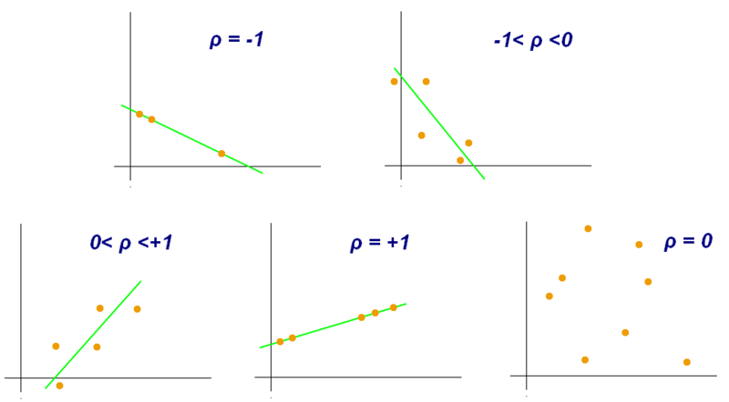
In particular, if our variables are named `x` and `y`, then

r = cov(x,y)/(sd(x) * sd(y))
= E((x - E(x)) * (y - E(y))) / sqrt[E((x - E(x))^2) * E((y - E(y))^2)]

where `E(x)` denotes the expected value of `x`.

However, this coefficient can only measure linear relationships, and fails miserably for non-linear relationships. That's where the Universal Correlation Coefficient comes in.

So, how does it work?

Well, let's do this by way of example. First, go ahead and load the library (follow the installation instructions on the GitHub README to install the library).

library(ucc)

Since this example will rely on randomly generated data, let's use the `set.seed()` function to set a particular seed for R's random number generator, and then pick 1000 randomly generated values uniformly selected between 0 and 1 for the variable `x`.

set.seed(1234)
x <- runif(1000)

Let's create two data sets: `dat_exact_fit` which contains points that perfectly lie on the curve `y = exp(x) * cos(2*pi*x)`, and `dat_xy` which contains points that are almost on the curve (ie we introduce some noise). We'll mostly be looking at `dat_xy`, but the exact fit data will also be useful to reference.

dat_xy <- data.frame(x=x,y=exp(x) * cos(2 * pi * x) + rnorm(1000,-0.1,0.1))
dat_exact_fit <- data.frame(x=x,y=exp(x) * cos(2 * pi * x))

If we look at a scatterplot of `dat_xy`, we see a (contrived) non-linear relationship:

plot(dat_xy,pch=20)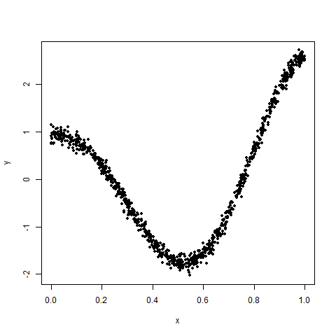

And, in fact, the Pearson correlation coefficient isn't helpful for this data, yielding a value of about `0.27`.

cor(dat_xy$x,dat_xy$y)
[1] 0.2666508

So, to get a coefficient that measures how close our data is to being on a curve (that may or may not be a line), we'll need to think a bit more generally. In particular, it will help us to move from specific `(x,y)` coordinates to ranks of `y` (in other words, the smallest `y` value has a rank of 1, the second lowest has a rank of 2, etc).

Why ranks? Well, go back to thinking about data that lies on a straight line with a positive slope. If we have `n` points in our scatterplot, then the `y` ranks--from left to right--are going to be `1,2,...,n`. In fact, this will be the case for data lying on any strictly increasing function of `x`. On the other hand, data lying on any strictly decreasing function of `x` will have the exact opposite rank set for `y`.

While this helps us sort out data that's close to being on curves that are functions of `x` and are either strictly increasing or strictly decreasing, we want to be even more general, so we instead look at absolute values of successive differences of ranks--ie the absolute value of the rank of the first `y` value minus the rank of the second `y` value, etc. For the case of strictly increasing or strictly decreasing data, all of these deltas are 1. And if our data looks like buckshot--ie no relationship whatsoever--then there will be a lot of variation in these deltas. This turns out to be our main insight and the motivation for the definition of the Universal Correlation Coefficient (which will be explicitly given below)

So, moving back to our data, our first transformation will be to sort it by `x` (in ascending order). There's a built-in function to do that, called `ucc.sort`.

dat_xy <- ucc.sort(dat_xy)

And a quick look reveals that our data seems to be sorted by `x` (the function `head()` only reveals the first six rows of our data):

$ dat_xy <- ucc.sort(dat_xy)
$ head(dat_xy)
x         y
783 0.0003418126 0.7482283
473 0.0006121558 1.1458113
746 0.0008630857 0.7665639
996 0.0013087022 0.9052347
383 0.0021467118 0.8658876
361 0.0031454624 0.8505322

(Note that you can ignore the column of numbers before the `x` values; those are the row numbers of `dat_xy` before we sorted it.)

The `ucc` library also has a built-in function to determine the ranks of `y`, called `ucc.ranks`.

$ head(ucc.ranks(dat_xy))
x   y
783 0.0003418126 709
473 0.0006121558 833
746 0.0008630857 716
996 0.0013087022 774
383 0.0021467118 759
361 0.0031454624 750

And the function for determining deltas--ie absolute values of successive ranks of `y` with respect to `x`--is `ucc.delta`. Note that this function returns a vector instead of a data frame.

$ ucc.delta(ucc.ranks(dat_xy))[1:5]
[1] 124 117  58  15   9

And, in fact, here is a plot of the deltas of ranks of `dat_xy`:

plot(ucc.delta(ucc.ranks(dat_xy)),pch=20
,ylab="deltas of y ranks w.r.t. x")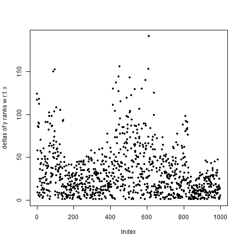

Now, this may initially look horrible: the deltas max out at over 150. However, these deltas are "squished" a lot farther down than if our data were random. In fact, let's go ahead and use a different random seed and generate another set of 1,000 random values.

set.seed(5678)
random_y = runif(1000)
dat_random <- data.frame(x=x,y=random_y)

Here's a scatterplot of `dat_random`:

plot(dat_random,pch=20)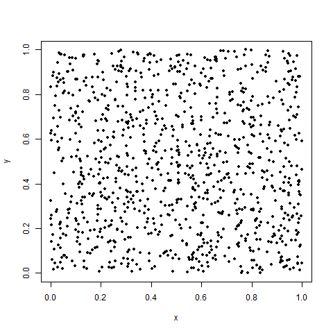

Yep. Buckshot. And here's a plot of the deltas of `y_random` with respect to `x`:

plot(ucc.delta(ucc.ranks(dat_random)),pch=20
,ylab="delta of random_y ranks w.r.t. x")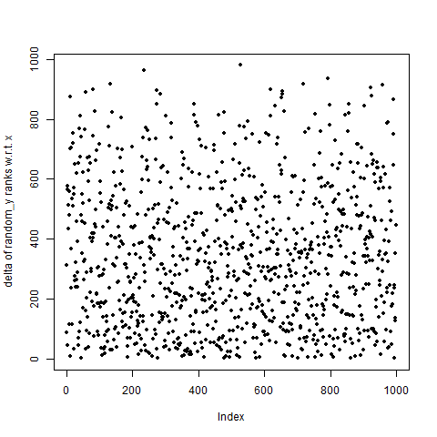

Still buckshot.

On the other hand, here's what the deltas look like for an exact fit:

plot(ucc.delta(ucc.ranks(dat_exact_fit)),pch=20
,ylab="delta of exact fit data y values w.r.t. x")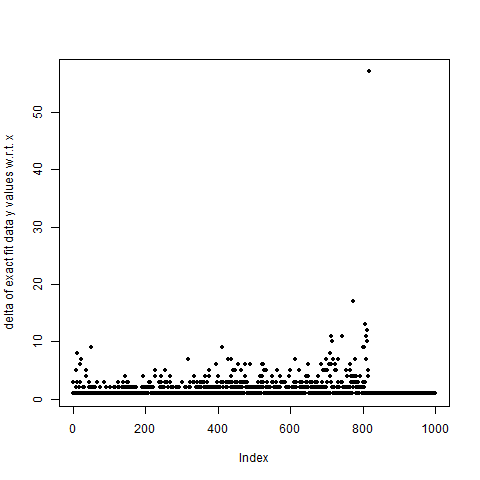

Definitely squished down a lot more!

All right, enough rambling, already. What exactly IS this Universal Correlation Coefficient?!

Let `a` denote the average of the delta of `y` ranks with respect to `x`. It turns out that `a` approximately equals `31.44`.

$ a <- mean(ucc.delta(ucc.ranks(dat_xy)))
$ a
[1] 31.44444

Now, imagine that the set of `y` ranks that we've found was randomly sampled out of all possible sets of `y` ranks for 1,000 different data points. For each possible set of ranks, we can compute the deltas and find the average of the deltas. So, the main question is how does `a` compare to `E(a)`, the expected value of delta averages across all sets of deltas?

Well, if we assume that these delta sets are independent and identically distributed, then it can be shown (using a bit of combinatorial finesse) that

E(a) = (n + 1) / 3

where `n` is the number of points in our data set. So, for `dat_xy`, we have `E(a) = 1001 / 3 = 333.67`. That's over ten times larger than `a`!

So, with all of this out of the way, we define

UCC_y = 1 - a / E(a) = 1 - (3 \* a) / (n + 1).

This represents the degree of dependency of `y` on `x`. Note that the smaller `a` is, the higher the coefficient (and the better the relationship). For `dat_xy`, we happen to have `UCC_y = 0.9057609`.

And if we start over again with `x` and `y` replaced (ie ordering by `y`, taking ranks of `x` with respect to `y`, taking the deltas, etc), we get

UCC_x = 1 - a / E(a) = 1 - (3 \* a) / (n + 1)

where this time, `a` is the average of the deltas of `x` with respect to `y`. `UCC_x` represents the degree of dependency of `x` on `y`. For `dat_xy`, we happen to have `UCC_x = 0.5447585` (which makes sense, since the curve upon which the data nearly fits doesn't form a function of `y`).

Finally, we define the universal correlation coefficient to be the maximum of the two coefficients above:

UCC = max(UCC_x,UCC_y)

And, of course, for `dat_xy`, we have `UCC = 0.9057609`, thus there's a strong relationship between these two variables.